Introduction
The IBM Data Analyst Professional Certificate on Coursera is a well-structured program designed to help learners develop the skills and knowledge required to succeed in data analysis. This course, created by IBM, offers practical training using real-world data and industry-standard tools, making it appealing for beginners and those looking to shift into a data-related career. Below is an in-depth review of the program.
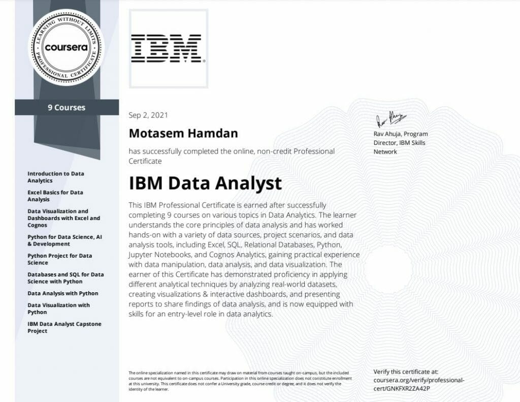
As I promised, I completed the IBM Data Analyst Professional Certificate and wanted to share my review in addition to course notes that will aid you in completing this career path.
Overview of the IBM Data Analyst Professional Certificate
- Duration: Approximately 3-6 months (depending on your pace)
- Number of Courses: 9 individual courses
- Skill Level: Beginner-friendly, no prerequisites required
- Mode: Online, self-paced
- Tools and Technologies Covered: Excel, SQL, Python, IBM Cognos Analytics, Jupyter Notebooks, Pandas (Python library)
IBM Data Analyst Course Components
The IBM Data Analyst Professional Certificate consists of 9 courses, each designed to build a foundation in data analysis through theoretical and practical lessons. Here’s a breakdown of the courses:
Course 1: Introduction to Data Analytics: A basic introduction to what data analysis is, the different roles in data science, and an overview of the analytics process.
Course 2: Excel Basics for Data Analysis: Teaches the essential skills needed to use Microsoft Excel for organizing, analyzing, and visualizing data. It includes formulas, functions, and pivot tables.
Course 3: Data Visualization and Dashboards with Excel and Cognos: Provides knowledge on how to create charts, graphs, and interactive dashboards using Excel and IBM’s Cognos Analytics.
Course 4: Python for Data Science, AI & Development: An introduction to Python programming focused on using the language for data science tasks.
Course 5: Python Project for Data Science: A project-based course where learners apply Python knowledge to solve a real-world data problem.
Course 6: Databases and SQL for Data Science: Teaches database concepts and how to use SQL to query and analyze databases.
Course 7: Data Analysis with Python: Covers the basics of using Python libraries like Pandas and Numpy for data wrangling and analysis.
Course 8: Data Visualization with Python: Introduces data visualization libraries such as Matplotlib and Seaborn to create compelling visualizations.
Course 9: IBM Data Analyst Capstone Project: A final project that allows learners to showcase the skills acquired throughout the program by working on a real-world dataset.
The Complete Data Analytics Notes Catalog
Who is This Certificate For?
- Career Changers: Those looking to transition into data analysis or a data-related field, especially beginners who want a solid foundation in data tools and techniques.
- New Graduates: Fresh graduates who are looking to add practical skills and certification to their resumes.
- Business Professionals: Individuals who work with data in roles such as marketing, finance, or operations and want to gain more formal training in data analysis.
Skills you will learn
- Microsoft Excel
- Python Programming
- Data Analysis
- Data Visualization (DataViz)
- SQL
- Data Science
- Spreadsheet
- Pivot Table
- IBM Cognos Analytics
- Dashboard
- Pandas
- Nump
You will also learn how to
-
Demonstrate proficiency in using spreadsheets and utilizing Excel to perform a variety of data analysis tasks like data wrangling and data mining
-
Create various charts and plots in Excel & work with IBM Cognos Analytics to build dashboards. Visualize data using Python libraries like Matplotlib
-
Develop working knowledge of Python language for analyzing data using Python libraries like Pandas and Numpy, and invoke APIs and Web Services
-
Describe data ecosystem and Compose queries to access data in cloud databases using SQL and Python from Jupyter notebooks
Jobs you can apply to after completing IBM Data Analyst
The skills taught in this course are highly relevant to the current job market, particularly for entry-level data analysts. Common roles that the program prepares learners for include:
- Data Analyst
- Junior Data Scientist
- Business Analyst
- Data Visualization Specialist
Cost and Value
- Cost: The program is accessible through Coursera’s subscription model, typically around $39-$49 per month, though Coursera often offers financial aid and free trials.
- Value: Given the extensive curriculum and the fact that it’s developed by IBM, the certificate offers good value for the cost, particularly if completed in a few months.
While the program is comprehensive for beginners, more advanced or niche roles in data science, like machine learning engineer or data architect, may require further training beyond this certificate.
Advantages of taking IBM Data Analyst by Coursera
Comprehensive Curriculum: The certificate offers a well-rounded introduction to the key aspects of data analysis, from Excel and SQL to Python programming and visualization techniques.
Hands-on Projects: Each course includes practical exercises and projects that allow learners to apply theoretical knowledge. The final capstone project is a great way to demonstrate your abilities in a real-world scenario.
IBM Branding: Being an IBM-developed program gives the course added credibility, and completing it provides learners with an IBM-branded certificate.
Flexible and Beginner-Friendly: The courses are self-paced, and there are no prerequisites, making it suitable for those new to data analysis.
Industry-Relevant Tools: The use of tools like Excel, SQL, Python, and IBM Cognos Analytics prepares learners for real-world data analysis tasks.
Limitations of IBM Data Analyst Professional Certificate
Limited Advanced Content: While the program does cover foundational concepts well, it may not delve deeply into more advanced topics like machine learning or advanced statistical methods, which some users may seek for more complex data roles.
Self-Paced Nature: While flexibility is a strength, some learners may struggle without deadlines or live interactions, which could impact their motivation and completion rates.
Cognos Analytics: While IBM Cognos Analytics is a useful tool, it is not as widely used in the data analysis industry as tools like Tableau or Power BI, limiting its direct applicability for some learners.
Certificate Recognition
The IBM Data Analyst Professional Certificate is widely recognized and respected by employers, particularly in entry-level data roles. Additionally, Coursera’s partnership with IBM enhances the certificate’s credibility. Many learners use this certificate as a stepping stone to more advanced certifications or degrees in data science.
Video WalkThroughs
Course Badge and Certificate
- Badge
- Certificate is below